CSP

Search can be for two different things:

• Search/Planning: Finding sequences of actions
  • The path to the goal is the important thing
  • Paths have various costs, deptsh
  • Heuristics give problem-specific guidance
• Identification: Assignments to variables
  • The goal itself is more important, not the path
  • All paths at the same depth (for some formulations)

Constraint Satisfaction Problems §

• Standard Search Problems
  • State is a “black box”: arbitrary data structure
  • Goal test can be any function over states
• Constraint satisfaction problems (CSPs): a special subset of search problems
  • State is defined by variables $X_i$ with values from a domain $D$
  • Goal test is a set of constraints specifying allowable combinations of values for subsets of variables
• Allows useful general-purpose algorithms with more power than standard search algorithms

CSP Example: Map Coloring §

Goal is to visualize different territories/regions. Each region should have different distinct colors. Kinda like 3-coloring from Algorithms

• Variables: WA, NT, Q, NSW, V, SA, T (shorthand of the region names)
• Domain: D = { red, green, blue }
• Constraints:
  • Implicit: WA =/= NT (regions next to each other shouldnt have the same color)
  • Explicit: (WA, NT) $\in$ { (red, green), (red, blue), … }
• Solutions are assignments satisfying all constraints e.g.
  • {WA=red, NT=green, Q=red, NSW=green, V=red, SA=blue, T=green}
  • There could be multiple solutions

CSP Example: Sudoku §

• Objective is to fill the empty cells with numbers between 1 and 9
• Numbers can only appear once in each row, column and box
• Variables? Domain?
• Variables $v_{ij}$ is the value in the jth cell of the ith row
• Domain $D=\{1,2,3,4,5,6,7,8,9\}$
• Constraints
  • Row Constraint: ${\forall }_i,\cup j\{v_{ij}\}=D$
  • Column Constraint: ${\forall }_j,\cup i\{v_{ij}\}=D$
  • Block Constraint: ${\forall }_K{\cup }_{(i,j)}\{v_{ij}|ij\in B_k\}=D$

Varieties of CSPs and Constraints §

Variables

• Discrete Variables
  • Finite domains (e.g., Boolean CSPs Boolean satisfiability)
    • Domain size $d$ and number of variables $n$ means $O(d^n)$ complete assignments
  • Infinite domains (e.g. job scheduling, variables are start hours for each job)
    • Linear constraints are solvable, nonlinear are undecidable
• Continuous variables (e.g. start precise times for Hubble Telescope observations)
  • Linear constraints solvable in polynomial time by linear programming (LP) methods Constraints
• Unary constraints involve a single variable (equivalent to reducing domains) for example $\text{SA}\ne \text{green}$
• Binary constraints involve pairs of variables e.g. $\text{SA}\ne \text{WA}$
• Higher order constraints involve 3 or more variables e.g. Sudoku row constraints
• Preferences (soft constraints)
  • e.g. red is better than green
  • Often representable by a cost for each variable assignment
  • Gives constrained optimization problems

Constraint Graphs §

• Binary cSP: each constraint relates (at most) two variables
• Binary constraint graph: nodes are variables, edges show constraints
• 
• The edges really say “WA =/= NT” for example
• General purpose CSP algorithms use the graph structure to speed up search
  • For example, Tasmania is an independent subproblem in the above graph

Solving CSPs §

• What if we used standard search formulation for CSPs
• States defined by the vlaues assigned so far (i.e. partial assignments)
  • Initial state; the empty assignment, {}
  • Action (successor function): assign a value to an unassigned varaible
  • Goal test: the current assignment is complete and satisfies all constraints
• However, these would result in very large search graphs where we check too many solutions, or don’t stop a solution early enough
• A naïve state space search has plenty of problems
• Backtracking Search
  • The basic uninformed algorithm for solving CSPs
  • Idea 1: One variable at a time
    • Variable assignments are commutative, i.e. [WA = red then NT = green] is the same as [NT = green then WA = red]
    • Fix ordering of variables and only consider assignmentsto a single variable at each step
  • Idea 2: Check constraints as you go
    • Incremental goal test i.e. consider only values which do not conflict previous assignments Might have to do some computation to check constraints
  • Depth-first search with these two improvements is called bcaktracking search
  • 
  • We don’t even branch down the path where both are red since it violates the constraint immediately

function backtracking-serach(csp) returns solution/failure
	return recursive-backgracking({}, csp)
function recursive-backtracking(assignment, csp) returns solution/failure
	if assignemnt is compelte then return assignment
	var <- selected - unassigned-variable(variables[csp], assignemnt, csp)
	for each value in order-domain-values(var, assignment, csp) do
		if value is consistent with assignment given constraints[csp] then
			add {var = value} to assignment
			result <- recursive-backtracking(assignment, csp)
			if result =/= failure then return result
			remove {var = value} from assignemnt
	return failure

Backtracking is DFS + variable ordering + fail on violation

• Improving Backtracking
  • There are some general purpose ideas that can result in huge gains in speed
  • Filtering
    • Can we detect inevitable failure early?
  • Ordering
    • Which variable should be assigned next?
    • In what order should its values be tried?
  • Structure
    • Can we exploit the problem structure?
• Filtering
  • Keep track of domains for unassigned variables and cross off bad options
  • Forward checking: cross offf values that violate a constraint when a value assignment is added to the existing assignment
  • 
  • As soon as WA is red, we get rid of red from NT and SA cuz they cant be red ever, no need to even consider it
  • If the domain of a variable is ever empty, we have a problem
  • 

Additional Heuristics §

Ordering §

In backtracking we have to select unassigned variables and loop through the order domain values. What order should we use for those?

• Ordering of variables - Minimum Remaining Values (MRV)
  • Order the variables on the number of remaining values in its domain
  • Also called the “most constrained variable”
  • “Fail-fast” ordering: if a partial assignment will fail, let it fail as early as possible
• Degree heuristic
  • What about the first variable we choose?
  • Degree heuristic: select the variable that is involved in the largest number of constraints
    • This will remove the most elements from the nearby domains
    • Makes the largest number of other variables more “constrained” and enable early falilures indirectly
    • 
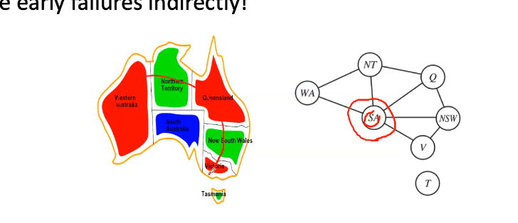
    • Choose South Australia to start since it affects the most things
• Ordering the values - Least Constraining Value (LCV)
  • Given a choice of variable, choose the least constraining value, i.e. the one that rules out the fewest values in the other unassigned variables
  • May take some computation to determine this (e.g. rerun filtering)

Improving Backtracking §

• Some general purpose ideas can result in huge gains in speed
• Filtering: Forward checking, constraint propagation, k-consistency
  • Can we detect inevitable failure early?
• Ordering
  • Which variable should be assigned next? MRV degree
  • In what order should its values be tried? LCV
• Problem Structure
  • Can we exploit the problem structure? Identify independent subproblems, leverage tree structures, cutset conditioning

Problem Structure §

• Sometimes we can have independent CSP subproblems within our main problem
• Independent subproblems are identifiable as connected components of constraint graph
  • Each subproblem can be solved independently
• Suppose a graph of $n$ variables with domain size $d$ can be broken into subproblems of only $c$ variables
  • Without decomposing: worse case solution cost is $O(d^n)$
  • With decomposing: $O((n/c)(d^c))$ linear in $n$

Tree-Structured CSPs §

• If the constraint graph has no loops (i.e. shows a tree structure) the CSP can ber solved in $O(n{d}^2)$ time
  • Compare to general CSPs where the worst case time is $O(d^n)$
  • 
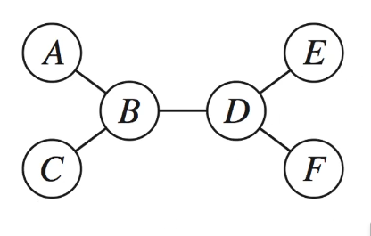
• Algorithm
  • Order: Choose a root variable, order variables so that parents precede children
  • 
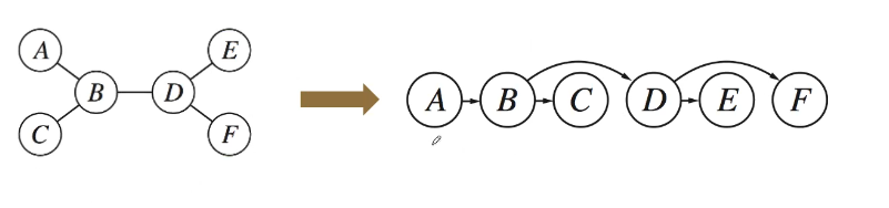
  • Enforce arc consistency (e.g. using the AC-3 algorithm) from the leaf to the root
    • Parent(X_i) -> X_i
    • Runtime: $O(n{d}^2)$

Nearly Tree-Structured CSPs §

• 
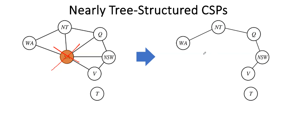
• Removing South Australia turns the subproblem in to a tree structure effectively
• Cutset: a set of variables such that after removing variables in this set and the constraints associated with the variables in this set, the constraint graph becomes a tree
  • In the example above it’d be SA
• Cutset conditioning: instantiate (in all ways) the variables in the cutset, update the domains for the remaining variables, and solve the CSP subproblem represented by the remaining constraint tree
• When the number of variables in the cutset size is $c$ the worst case runtime is $O((d^c)(n-c)d^2)$
  • very fast for small $c$

Iterative Algorithms for CSPs §

• Local Search methods typically work with “complete” states, i.e. all variables are assigned
• To apply to CSPs
  • Take an assignment with unsatisfied constraints
  • Operators reassign variable values
• Algorithm sketch:
  • While CSP is not solved; Variable selection: randomly select any conflicted variable Value selection: min-conflicts heuristic (choose a value that violates the fewest constraints) effectively hill climb with h(n) = total number of violated constraints