The search methods in Search Problems
- systematically explore the full search space
- return the path from start node to the goal But in many problems, the path is irrelevant; the goal state itself is the only thing we care bout
- 8-Queens problems Sometimes the goal test itself is unclear, i.e. you are really solving an optimization problem
- Traveling Salesperson
- Given a list of cities and the distances between each pair of cities, what is the shortest possible route that visits each city exactly once and returns to the origin city? This leads to Local Search
Discrete State Space
- Local search is useful when the path to the goal state does not matter or you are solving a pure optimization problem
- Basic idea:
- only keep a single “current” state
- Try to improve iteratively
- Don’t save paths followed
- Characteristics
- Low memory requirements - usually constant
- Effective - can often find good solutions in extremely large state spaces
- Example: Eight-queens problem
- Place eight queens on a chessboard so that no queen can attack another
- We can formulate the search with
- Incremental formulation
- Complete-state formulation
- Heuristic/Objective: number of pairs of attacking queens (when this is 0 we are at a goal state, there’s no queens attacking each other. Satisfies Heuristic requirements)
Hill-Climbing Search
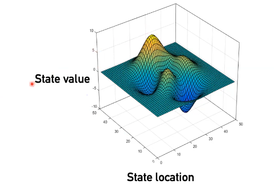
- Consider a state-space landscape where:
- Location = state
- Elevation = evaluation of state (objective function value)
- Continually move in the direction of increasing value (if trying to maximize objective function)
- Think finding the a local maximum on a 3 dimensional graph/plane like this
function HillClimbing(problem) return a state that is a local maximum
	current <- initial_state
	repeat:
		best_neighbor <- current
		for state in Neighbors(current):
			if state.value > best_neighbor.value:
				best_neighbor <- state
		if best_neighbor.value > current.value
			current <- best_neighbor
		else:
			return current
- Challenges for hill-climbing
- Once a local maximum is reached, there is no way to backtrack or move out of that maximum
- Hill-climbing can have a difficult time finding its way off a flat portion of the state space landscape
- Ridges can produce a series of local maxima that are difficult to navigate out of
Variants of local hill-climbing
- Stochastic hill-climbing
- Select randomly from all moves that improve the value of the objective function
- Random-restart hill-climbing
- Conduct a series of hill climbing searches, starting from random positions
- Very frequently used general method in AI
Simulated Annealing
- inspired by statistical physics/metallurgy
- Key idea: mostly goes “uphill” but ocassionaly travels “downhill” to escape the local optimum
- The likelihood to go downhill is controlled by a “temperature schedule”
- more and more “conservative” i.e. less likely to go downhill as the search progresses
function SimulatedAnnealing (problem, schedule) return a solution state
	current <- initial_state;
	for t=1 to infinity:
		T <- schedule(t)
		if T = 0 then return current
		next <- a randomly selected neighbor of current
		deltaE = next.value - current.value
		if deltaE > 0:
			current <- next
		else:
			current <- next with probability e^{deltaE / T}
Local beam search
- Similar to hill climbing but
- Keeps track of current states rather than just a single current state
- Select the best neighbors among all neighbors of the k current states
- Can be combined with stochastic for stochastic beam search
Genetic Algorithm
- Inspired by evolutionary biology
- Mimic the evolution of a population under natural selection: the fittest survives (i.e. the ones with better objective function values)
