Search Problems

Assumptions on the task environment for search problems:

• Fully observable - States can be fully determined by observations
• Single agent - Only one agent is involved
• Deterministic - The outcomes of actions are certain
• Static - The world does not change on its own
• Discrete - A finite number of individual states exist rather than a continuous space of options
• Known - The result of actions are known
  

Claim: Many problems faced by intelligent agents, when properly formulated, can be solved by a single family of generic approaches: search

Definitions §

• States: $s$, that describe the configuration of the environment
• Initial state: $s_0$, the state that an agent starts in
• Actions (operators): $a$, activities which move the agent from one state to another
  • Actions(s) returns a finite set of actions that can be executed in state s
• Transition model (successor function): Describes what each action does
  • Result(s, a) returns the state that results from doing action a at state s
• State space: the set of states reachable from the initial state by applying any sequence of actions
  • State space is usually represented as a graph
• Goal state: A set of possible states to reach
  • IsGoal(s) indicates whether a state s is a goal state
• Step/Action Cost: ActionCost(s, a, s’) the cost of taking an action a which moves the agent from state s to s’
• Path: a sequence of actions
• Path cost: the cost of a path
• Solution: a path from the initial state to a goal state
  • Quality of a solution is measured by its path cost
• Optimal solution: any solution with the lowest path cost
• Search algorithm: the algorithm that determines which actions should be tried in which order to find a path from the initial state to a goal state
• Model: an abstract mathematical description of a real world problem
• Abstraction: the process of removing details from a representation

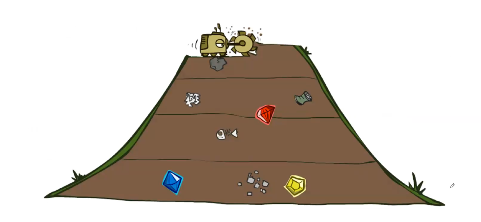
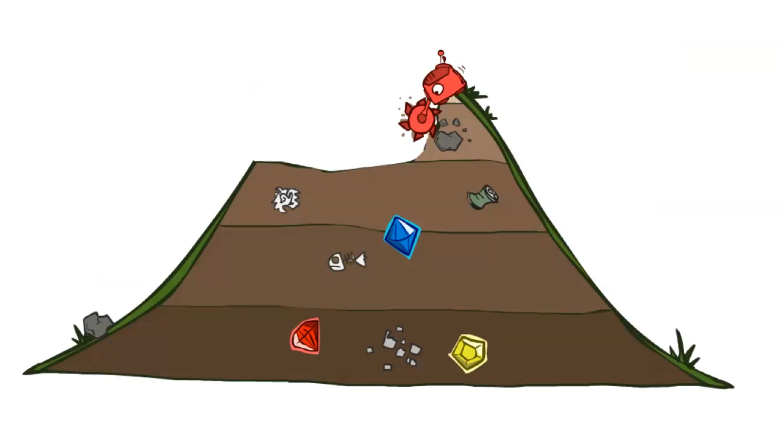
Example Problems §

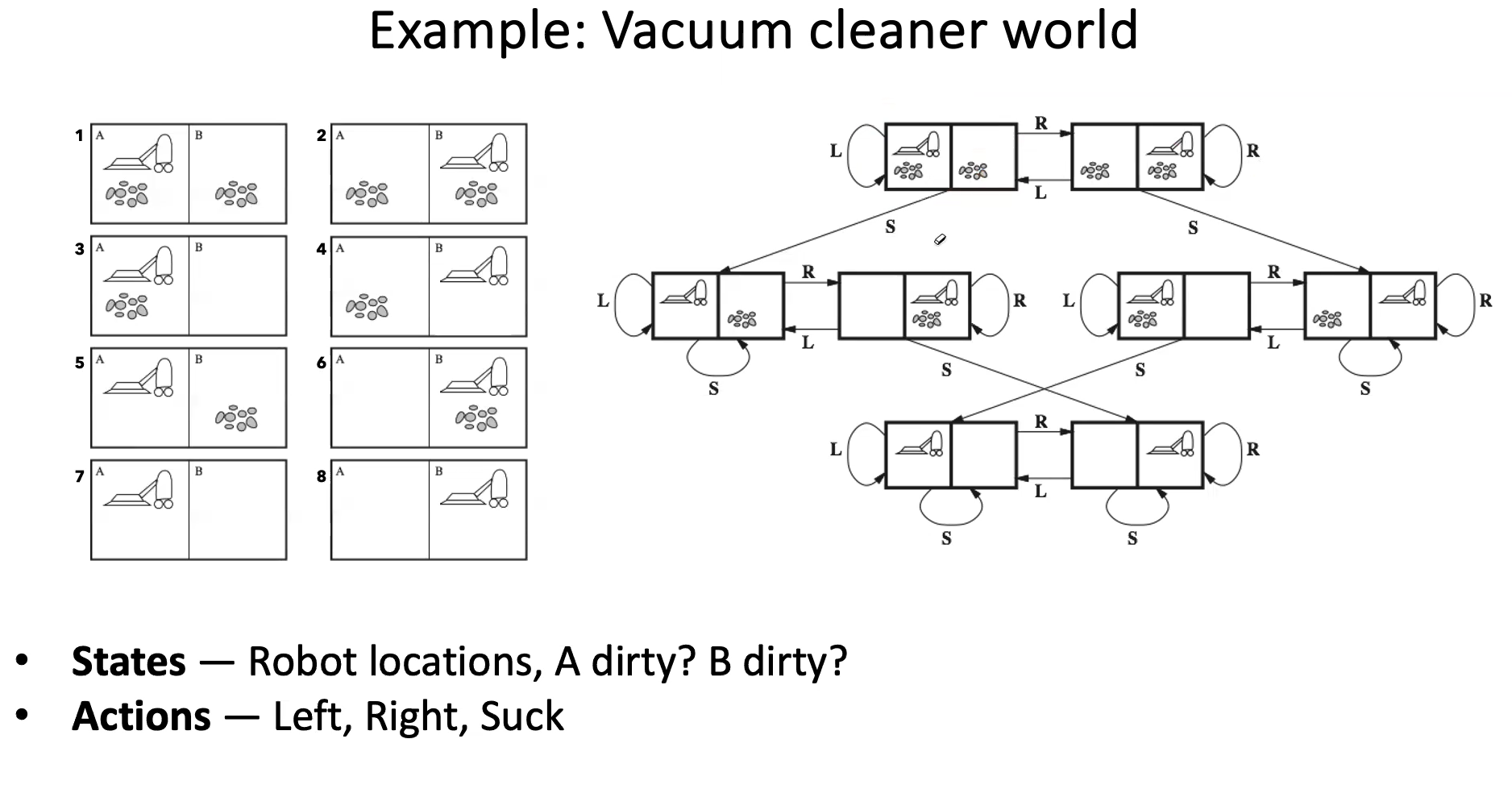On the left is just the atomic states. The right shows the relationship between each state and actions to get from one state to another.

• Goal test - no dirt
• Path cost - 1 per operation
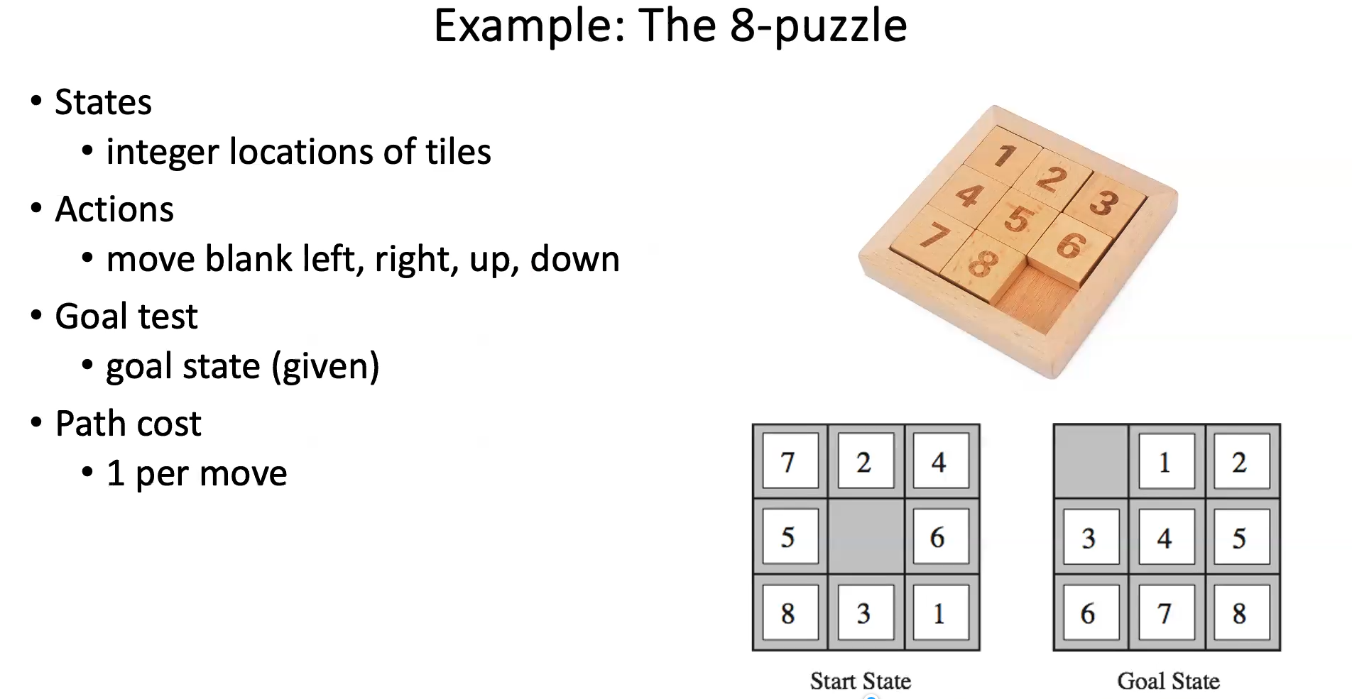
• You could make the actions move each tile but that makes the number of actions WAY bigger than it needs to be
• Moving just the blank is less actions but same resultant states

Search Algorithm §

• A search algorithm takes a search problem as input and returns a solution
• State space graphs are mathematical representations of a search problem
  • Nodes are (abstracted) world configurations
  • Edges represent successors (results of actions)
  • Look at vacuum cleaner example above
  • The goal test is a set of goal nodes (maybe only one)
  • In a state space graph, each state occurs only once
  • We can rarely build this full graph in memory due to size, but its a useful idea
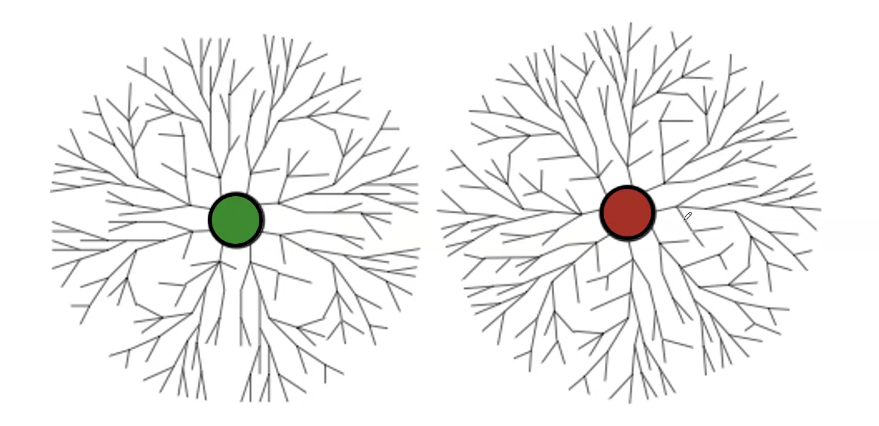
• Another useful concept is a Search Tree
  • A “what if” tree of actions and their outcomes
  • Root node = initial state
  • Children correspond to successors based on different actions
  • Nodes show states, branches correspond to actions that lead to those states
  • For most problems, we can never actually build the whole tree

General Tree Search Algorithm Pseudocode §

function TreeSearch(problem) return a solution, or failure
	frontier <- {initial_state}
	repeat
		if frontier is empty then return failure
		node <- POP(frontier) 
		// Search alogirhtms differ in how they pick the next node to expand from the frontier
		if IsGoal(node) then return the corresponding solution
		for a in Actions(node):
			s' = Result(node, a)
			INSERT(frontier, s')

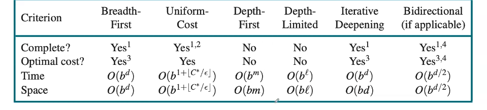
Uniform Search §

An uninformed search algorithm has no additional information about states beyond what has been provided in the problem formation

• Depth-first search

  • 
  • Strategy: expand the deepest node first
  • Depth is the # of actions in a path (node)
  • Time complexity
    • DFS could process the whole tre (and the depth could be greater than the shortest depth goal)
    • if m is finite, takes time $O(b^m)$
  • Space complexity
    • only need to store siblings on path to m tiers root, so $O(bm)$
  • Is it complete?
    • If the depth is infinite then no (i.e. the path you take has you constantly going left but the solution is just 1 right)
  • Is it optimal?
    • No, it finds the “leftmost” solution, regardless of depth or path cost

• Breadth-first search

  • 
  • Strategy: expand the shallowest node first
  • Depth is # of actions in a path (node)
  • can be implemented with a FIFO Queue
  • Time complexity
    • BFS processes all nodes above shallowest solution
    • Let depth of shallowest solution be $d$ and $b$ be the number of “branches” each node has
    • Search takes time $O(b^d)$
  • Space complexity
    • Needs to store roughly the successors of the last tier, so $O(b^d)$
  • Is it complete?
    • Yes, $d$ must be finite if a solution exists
  • Is it optimal?
    • Only if costs are all 1 BFS will outperform DFS when the goal is shallow. DFS outperforms when the space complexity is constrained.
      

• Depth-limited search

  • Add an arbitrary limit so if the depth gets to $l$ than we terminate with failure

• Iterative deepening depth-first search

  • Get DFS’s space advantage with BFS’s time/shallow-solution advantages
  • Run a DLS with depth limit 1, if no solution…
  • Run a DLS with depth limit 2. If no solution…
  • Run with depth 3…
  • Gives the space complexity benefits of DFS but the searching of BFS
  • Generally the most work happens in the bottom level searched so its not really too badz

• Bi-directional search

  • 
  • Search from both ends
  • Desirable when $O\left(b^{\frac{d}{2}}\right)+\left(b^{\frac{d}{2}}\right)<O(b^d)$
  • Need to know the goal state though before you start searching

• Uniform-cost search

  • 
  • Strategy: expand the cheapest node first
  • Implementation is make the frontier a priority queue using the cumulative cost
  • Time Complexity
    • Processes all nodes with cost less than the cheapest solution
    • If that solution costs $C^{\ast }$ and actions at least $e$ then the “effective depth” is roughly $C^{\ast }/e$
    • Takes time $O(b^{1+[C^{\ast }/e]})$
  • Space complexity
    • Has roughly the successors of the last tier, so $O(b^{1+[C^{\ast }/e]})$
  • Is it complete?
    • Yes, assuming the best solution has finite cost and min action cost is positive
  • Is it optimal?
    • Yes All these search algorithms rely on some kind of Queue or Stack especially a priority queue (you can use a priority queue to act as a stack with smart priority setting)

• Best First Search (Generalized of the above searchs)

  • Choose a node $n$ with minimum value of some evaluation function $f(n)$
  • Priority queue ordered by $f$
  • Example: Breadth-first search: Expand the shallowest node first
    • $f(n)=\text{Depth}(n)$

Informed Search §

• The search algorithm uses domain specific hints about the location of goals (beyond the problem formulation)
• These hints are formularized through a heuristic function $h(n)$
• $h(n)$ is the estimated cost of the cheapest path from the state at node n to a goal state
• Idea: Best-First Search where $f(n)$ contains $h(n)$
• Heuristic Functions
  • Heuristic functions need to be non negative and need to somehow estimate how close a state is to a goal, designed for a particular problem
  • $h(n)=0$ if $n$ is a goal state
  • Examples: Manhattan distance, Euclidean distance for pathing

Greedy Search §

• Choose $f(n)=h(n)$
• Expand the node that SEEMS closest…
• Does not always get the optimal solution though
• Strategy: Expand a node that you think is closest to a goal state
• Heuristic: estimate of distance to nearest goal for each state
• Common case: Best-first takes you straight to the (wrong) goal
• Worst-case: like a badly guided DFS (with a poorly designed Heuristic)

A* Search §

• Basing purely on the heuristic doesn’t work perfectly, so why not include the path cost too?
• $f(n)=g(n)+h(n)$
  • $g(n)$ = path cost from start node to current node n
  • $h(n)$ = estimate of path cost from $n$ to the goal
• Expands the node $n$ if the estimated cost of the solution passing through it is the lowest
• Combines uniform cost search and greedy search
• A* search is optimal if $h(n)$ is an UNDERESTIMATE of the actual cost from $n$ to the goal
• When should A* terminate?
  • It shouldn’t immediately terminate when it finds a goal state
  • No, only stop when a goal state is EXPANDED (i.e. it exits the frontier)
• Is A* Optimal?
  • Not always. The Heuristic can be wrong.
  • We need the estimated costs $h(n)$ to be less than actual costs
  • It is optimal if the heuristic is admissible (see below)

Heuristics §

• A heuristic $h$ is admissible (optimistic) if $0\le h(n)\le h^{\ast }(n)$ where $h^{\ast }(n)$ is the true cost to a nearest goal
• Designing admissible heuristics is most of what’s involved in using A* in practice
• Creating Admissible heuristics
  • Most of the work in solving hard search problems is in designing admissible heuristics
  • Often, admissible heuristics are solutions to relaxed problems, where new actions are available
    • For example, in the Pacman maze problem, an admissible heuristic would be the Manhattan Distance (just go left and then go down). It basically treats the world as if there was no walls, which is a relaxed version of the true problem
  • Inadmissible heuristics are often useful too

Graph Search §

• Tree searches fail to detect repeated states, which can cause exponentially more work
• In a graph search we never expand a state twice
• We implement it by doing the same thing as tree search but also keep a list of the already expanded states (visited)
• Before expanding a node we check to make sure its state has not been visited
• If its not new, we skip it, if new we add to the visited set
• Its important to store the visited set as a SET not just a list
• Graph Search + Uniform Cost = Dijkstra’s Algorithm

General Graph Search Algorithm §

	frontier <- {initial_state}; explored <- empty set
	repeat
		if frontier is empty then return failure
		node <- POP(frontier) 
		// Search alogirhtms differ in how they pick the next node to expand from the frontier
		if IsGoal(node) then return the corresponding solution
		if node not in explored:
			explored.add(node)
			for a in Actions(node):
				s' = Result(node, a)
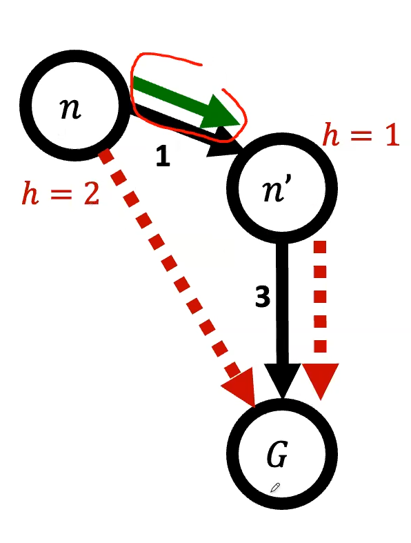
				INSERT(frontier, s')

In an A* graph search, we might run into issues. See the example below.

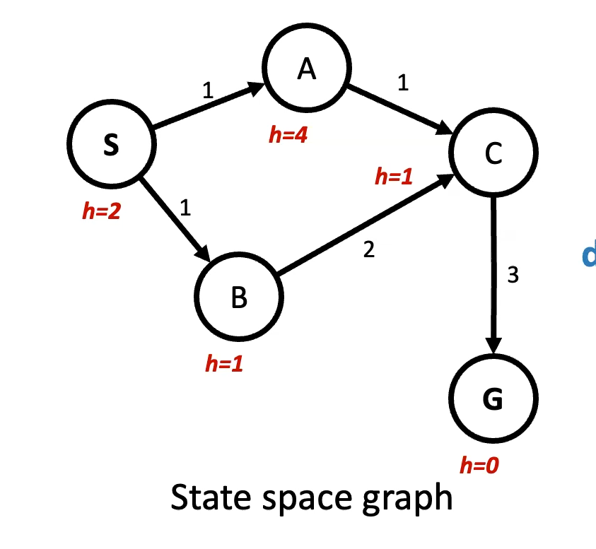
In order to keep A* optimal for Graph Search, we need to also make heuristics consistent

Consistency of Heuristics §

The estimated heuristic costs need to be less than or equal to the actual costs

• Admissibility: heuristic cost $\le$ actual cost to goal
  • $h(n)\le$ actual cost from n to G
• Consistency: heuristic “arc” cost $\le$ actual cost for each arc
  • $h(n)-h(n^{\prime })\le \text{cost}(n\text{ to }{n}^{\prime })$
  • $h(n)\le \text{cost}(n\text{ to }{n}^{\prime })+h(n^{\prime })$
• Formally a heuristic $h(n)$ is consistent, if for every node $n$ and ever successor $n^{\prime }$ of n
  • $h(n)\le \text{cost}(n\text{ to }{n}^{\prime })+h(n^{\prime })$
• Consistency IMPLIES admissibility